When learning something new, we tend to understand it from the perspective of something with which we are already familiar. We can approach a problem in so many ways, but one of the most important things I learned in my degree was to classify a problem before establishing a direction for its solution.
We can find classification everywhere in mathematics and statistics:
- Set theory categorises objects into sets
- Group theory generalises complex structures into groups
- Category theory uses contextual information to put things into categories
- Probability theory uses probability distributions to predict the occurrence of events
Each set, group, category and probability distribution have defined assumptions, boundaries on their operations and spaces of possible outcomes.
Classifying the classifier
Recently, I was part of a big data project where my group and I were using machine learning to predict the success or failure of a Kickstarter project. This problem reminded me of a previous project I had worked on at the very beginning of my career, where I was required to classify financial transactions associated with criminal or non-criminal activity:
- Both problems had predictor variables
- Both problems had a response variable with a binary class structure
- The odds of those classes were imbalanced—Kickstarter project success was rarer than its failure, just as financial crime activities were rarer than non-criminal activities
Immediately, I began to think of algorithms used for binary classification which could handle imbalanced classes in training. Why? Because algorithm suitability matters, and you will inevitably be questioned on your logical reasoning for every choice made in a project. As in mathematics and statistics, data science algorithms also have underlying assumptions defining their fit for a task.
In this article, we will explore the characteristics that help us classify a machine learning problem. This will lay the foundation for algorithms we can use and appropriate metrics for their evaluation. We will be diving into the space of possible algorithms and metrics for each type of machine learning method in future articles.
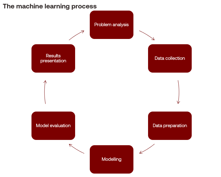
The machine learning process
Machine learning is a branch of artificial intelligence (AI) referring to the collection of algorithms that use data to discover patterns and relationships.
A machine learning algorithm is a step-by-step process to solve a problem. These algorithms calibrate their processes on a portion of the data called a training set. A machine learning model is the output of an algorithm trained on these data. Model fitness refers to how well a model generalises to unseen data; usually, the remaining portion of the data is called a test set.
At its core, the machine learning process is much like the data visualisation process in that it follows the scientific method.
- Performing a problem analysis: Formulating a question, developing null and alternative hypotheses.
- Collecting data: Finding information sources, acquiring relevant data and understanding it.
- Preparing data: Analysing the data, dealing with duplicate or incomplete information, fixing inaccuracies, removing irrelevant information, or augmenting data through feature engineering.
- Modelling: Selecting an algorithm based on its appropriateness to the method, training the algorithm on the input data and tuning it to develop a model.
- Evaluating the model: Selecting appropriate evaluation functions to estimate model fit.
- Presenting: Interpreting the results of the model, reporting to stakeholders.
Types of machine learning problems
There are three main types of machine learning problems: supervised learning, unsupervised learning, and reinforcement learning.
Supervised learning
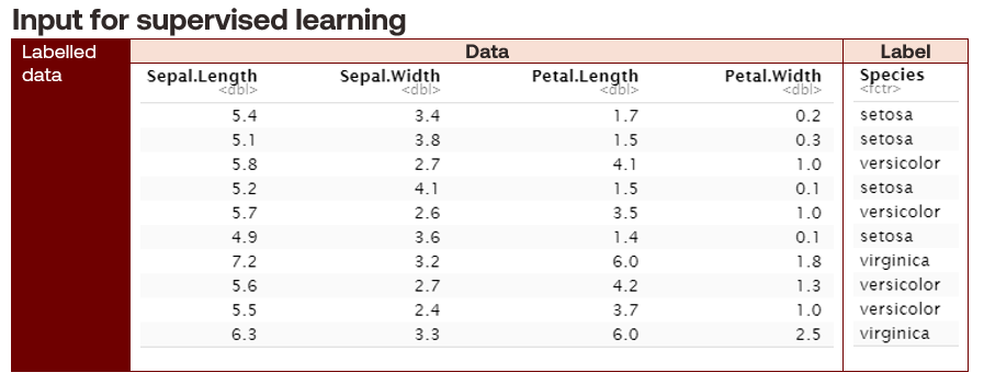
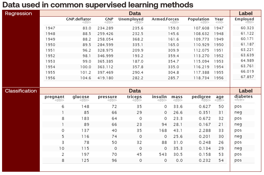
Supervised learning problems take labelled data as input to train algorithms to predict or classify outcomes. Labelled data describes training datasets containing a response variable. Some methods associated with supervised learning are regression and classification.
Unsupervised learning
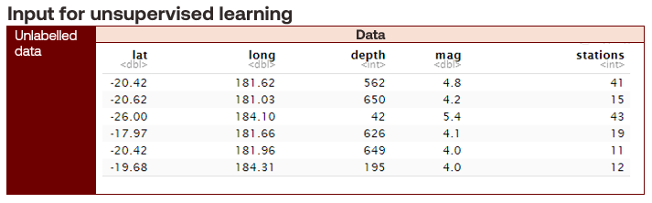
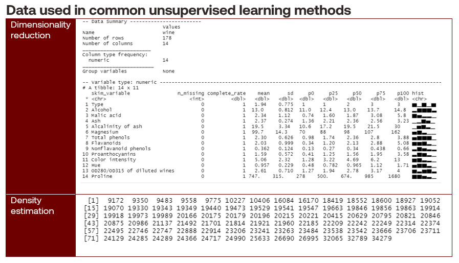
Unsupervised learning problems take unlabelled data as input and discover patterns within them. Unlabelled data describes training data sets that do not contain a response variable. Common methods include dimensionality reduction and density estimation.
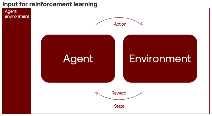
Reinforcement learning
Reinforcement learning problems are when an intelligent agent learns by trial and error using feedback from an interactive environment. The agent learns through rewards and punishments for positive and negative behaviour toward its goal, maximising its cumulative compensation. An example algorithm is the Monte Carlo method.
We will visit reinforcement learning much later in this series.
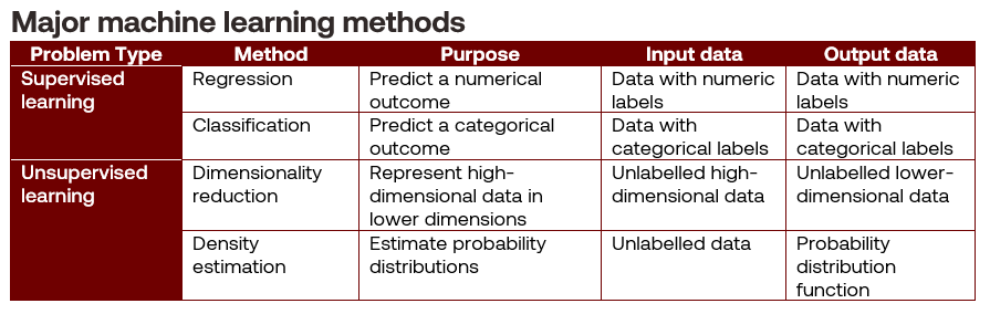
Types of machine learning methods
The following are four of the main methods that underpin many machine learning problems.
Supervised learning methods
Regression techniques use labelled data to predict a numerical outcome (except for the special case of logistic regression, which we will touch on in a future article). An example of this is predicting employment rates from economic variables. Expressed mathematically, a regression problem takes on the form:

Classification techniques use labelled data to predict a categorical outcome, such as separating a collection of objects into defined classes. These classes can be binary, such as the onset of diabetes from medical record data, or multi-class, such as the species of an iris flower. Mathematically, a classification problem is expressed:

Unsupervised learning methods
Dimensionality reduction techniques simplify higher-dimensional unlabelled data into lower-dimensional forms while retaining most of the information, such as estimating wine quality from sensor data. Dimensionality reduction is often used in the data preparation phase to improve model fit. Expressed mathematically, we want to find lower-dimensional projections:

Density estimation techniques are concerned with estimating the probability distributions of unlabelled data, such as finding galaxy clusters. An example of density estimation is Gaussian mixture models (GMM) that express a single distribution as a combination of K Gaussian distributions, as follows:

Conclusions
Machine learning refers to the collection of step-by-step processes called algorithms to solve a problem. Supervised learning problems predict outcomes from labelled data, whereas unsupervised learning problems discover patterns and relationships in unlabelled data. Reinforcement learning problems involve an intelligent agent learning from its environment.
If a supervised learning problem predicts a numerical response, we can use regression techniques; if it predicts a categorical response, we can use classification techniques. If an unsupervised learning problem has too many variables, we can use dimensionality reduction techniques. If we want to find a probability distribution, we can use density estimation techniques.
Just as we can classify sets, groups, categories and probability distributions into spaces with defined operations and possible outcomes, we can categorise machine learning problems and their methods, as shown in Table 3.